Lesson 03: MATLAB Matrices
Objective
- To understand and manipulate matrices
- To learn how to extract data from matrices
- To learn how to create and use special matrices
Background
When you use MATLAB to solve some complicated problems, you will find that you may need to create some small matrices, combine them into large matrices, extract data from the matrices, or create very large matrices.
3.1 Defining Matrices and Indexing Matrices
Defining Matrices
Defining Matrices
To define a matrix in MATLAB, you can:
- Type in a list of numbers enclosed in square brackets [ ]
- Column separator: use space or commas to separate elements of a column (you can even combine the two column separators in the same matrix definition)
>> A = [3 5]; B = [1.2, 3.3];
>> C = [1.5, 3.1 2.0 -0.5]; - Row separator: use semicolon (;) to indicate the end of each row
>> D = [-1, 0, 0; 1, 1, 0; 0, 0, 2];
- Column separator: use space or commas to separate elements of a column (you can even combine the two column separators in the same matrix definition)
- List each row on a separate line
>> E = [-1, 0, 0;
1, 1, 0;
1, -1, 0;
0, 0, 2]; - List each row on a separate line without the semicolon
>> E = [-1, 0, 0
1, 1, 0
1, -1, 0
0, 0, 2]; - Continue a long row number to the next line using ellipsis (...)
>> F = [1, 52, 64, 197, 42, -42, 55, 82, 22, 109]; #or
>> F = [1, 52, 64, 197, 42, -42, ...
55, 82, 22, 109]; - Create an empty matrix
>> G = [];
All the matrices must be rectangular (set undefined elements to zero).
Indexing Matrices
Accessing Elements
The following ways are how to access elements in a multidimensional array.
Indexing Matrices
Indexing into a matrix is a means of selecting a subset of elements from the matrix. MATLAB has several indexing styles that are not only powerful and flexible, but also readable and expressive. Indexing is a key to the effectiveness of MATLAB at capturing matrix-oriented ideas in understandable computer programs.
MATLAB indices start from 1. (In C, the index number of an array starts from 0).
$A = \left[ {\begin{array}{ccccccccccccccc} 1&2&3\\ 4&{ - 5}&6\\ 5&6&7 \end{array}} \right]$
|
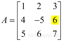
Indexing using parentheses |
|
| >> A(2,3) ans = 6 |
 |
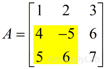
| Indexing submatrices using vectors of row and column indices | |
| >> A([2 3],[1 2]) ans = 4 -5 5 6 |
 |
| Ordering of indices is important! For example: | |
| >> B=A([3 2],[2 1]) # or >> B=[A(3,2),A(3,1);A(2,2),A(2,1)] B = 6 5 -5 4 |
 |
Colon (:) Operator
Colon (:) Operator
The colon operator is one of the most operators in MATLAB. It can create vectors, subscript arrays, and specify for-loop iterations.
Create Sequence Row Vector
x = firstVal : lastVal
Create a row vector of number between firstVal and lastVa. If ( firstVal > lastVal ), x will be assigned to an empty vector.
Create a unit-spaced vector of numbers between 1 and 10. The colon operator uses a default increment of +1.
>> x = 1:10
x = 1 2 3 4 5 6 7 8 9 10
x = firstVal : incr : lastVal
Create a row vector of number between firstVal and lastVal with increment incr.
Create a vector whose elements increment by 0.1.
>> x = 0 : 0.1 : 1
x = 0 0.1000 0.2000 0.3000 0.4000 0.5000 0.6000 0.7000 0.8000 0.9000 1.0000
Create a vector whose elements decrement by -2.
>> y = 10 : -2 : 0
y = 10 8 6 4 2 0
Common indexing expressions that contain a colon are:
- A(:,n) is the nth column of matrix A
- A(m,:) is the mth row of matrix A
- A(:,:,p) is the pth page of three-dimensional array A
- A(:) reshapes all elements of A into a single column vector. This has no effect if A is already a column vector
- A(:,:) reshapes all elements of A into a two-dimensional matrix. This has no effect if
Ais already a matrix or vector - A(j:k) uses the vector j:k to index into A and is therefore equivalent to the vector [A(j), A(j+1), ..., A(k)]
- A(:,j:k) includes all subscripts in the first dimension but uses the vector j:k to index in the second dimension. This returns a matrix with columns [A(:,j), A(:,j+1), ..., A(:,k)]
Index Matrix Rows and Columns
Examine several ways to index a matrix using a colon :
$A = \left[ {\begin{array}{ccccccccccccccc} 1&2&3\\ 4&{ - 5}&6\\ 5&6&7 \end{array}} \right]$
Index complete row or column using the colon operator, also can add limit index range.
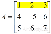
| Extract the first row: | |
| >> A(1,:) ans = 1 2 3 |
 |
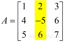
| Extract the second column | |
| >> A(:,2) ans = 2 -5 6 |
 |
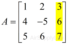
| Extract the last column | |
| >> A(:,end) ans = 3 6 7 |
 |
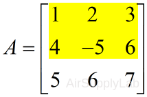
| Index the the first and second row | |
| >> A(1:2,:) # or >> A([1 2],:) ans = 1 2 3 4 -5 6 |
 |
| Index submatrices using limit range of row and column | |
| >> A(2:3 , 1:2) # or >> A([2 3],[1 2]) ans = 4 -5 5 6 |
 |
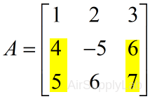
| Extract the first and third column from second and third row | |
| >> A(2:3 , 1:2:3) # or >> A([2 3],[1 3]) ans = 4 6 5 7 |
 |
Reshape the matrix
$A = \left[ {\begin{array}{ccccccccccccccc} 1&2&3\\ 4&{ - 5}&6\\ 5&6&7 \end{array}} \right]$
Reshape the matrix into a column vector.
>> A(:)
ans =
1
4
5
2
-5
6
3
6
7
Linear Indexing
Linear Indexing
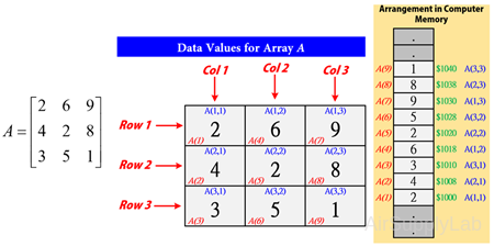
In MATLAB, arrays are stored in column-major order. It means that when a multi-dimensional array, its 1-D representation is the actually order stored in memory.
>> A = [2 6 9; 4 2 8; 3 5 1];
>> A(:)
A = 2, 4,, 3, 6, 2, 5, 9, 8, 1
The element at row 3, column 2 of matrix A (A3,2 = 5) can also be identified as element 6 in the actual storage sequence. To access this element, you have a choice of using the standard A(3,2) syntax, or you can use A(6), which is referred to as linear indexing.
Logical Indexing
Logical Indexing
Another indexing variation, logical indexing, has proven to be both useful and expressive. In logical indexing, you use a single, logical array for the matrix subscript. MATLAB extracts the matrix elements corresponding to the nonzero values of the logical array. The output is always in the form of a column vector. For example, A(A > 12) extracts all the elements of A that are greater than 12.
>> A( A > 12)
ans =
16
14
15
13
Many MATLAB functions that start with return logical arrays and are very useful for logical indexing. For example, you could replace all the NaN elements in an array with another value by using a combination of isnan, logical indexing, and scalar expansion. To replace all NaN elements of the matrix B with zero, use
>> B( isnan(B)) = 0
Sum of Array Element
The sum of array elements
| sum(A) | Returns the sum of A elements along the first array dimension whose size is greater than 1. |
| sum(A, "all") | Returns the sum of all elements of A. |
| sum(A, dim) | Returns the sum along dimension dim. For example, if A is a matrix, then sum(A,2) returns a column vector containing the sum of each row. |
| sum(A, vecdim) | Sums the elements of A based on the dimensions specified in the vector vecdim. For example, if A is a matrix, then sum(A,[1 2]) returns the sum of all elements in A because every matrix element is contained in the array slice defined by dimensions 1 and 2. |
| sum(___,outtype) | Returns the sum with the specified data type using any input arguments in the previous syntaxes. outtype can be "default", "double", or "native". |
| sum(___,nanflag) | Specifies whether to include or omit NaN values in A. For example, sum(A,"omitnan") ignores NaN values when computing the sum. By default, sum includes NaN values. |
Sum of Vector Elements
Create a vector and compute the sum of its elements.
>> A = 1:10;
>> S = sum(A)
S = 55
Sum of Matrix Columns
Create a matrix and compute the sum of the elements in each column.
>> A = [1 3 2; 4 2 5; 6 1 4]
A =
1 3 2
4 2 5
6 1 4
>> S = sum(A)
S =
11 6 11
Sum of Matrix Rows
Create a matrix and compute the sum of the elements in each row.
>> A = [1 3 2; 4 2 5; 6 1 4]
A =
1 3 2
4 2 5
6 1 4
>> S = sum(A,2)
S =
6
11
11
Sum of Array Slices
Use a vector dimension argument to operate on specific slices of an array.
Create a 3-D array whose elements are 1.
> A = ones(4,3,2);
To sum all elements in each page of A, specify the dimensions to sum (row and column) using a vector dimension argument. Since both pages are a 4-by-3 matrix of ones, the sum of each page is 12.
>> S1 = sum(A,[1 2])
S1 =
S1(:,:,1) = 12
S1(:,:,2) = 12
If you slice A along the first dimension, you can sum the elements of the resulting 4 pages, each 3-by-2 matrices.
>> S2 = sum(A,[2 3])
S2 =
6
6
6
6
Slicing along the second dimension, each page sum is over a 4-by-2 matrix.
>> S3 = sum(A,[1 3])
S3 = 8 8 8
To compute an array's sum overall dimensions, you can specify each dimension in the vector dimension argument or use the "all" option.
>> S4 = sum(A,[1 2 3])
S4 = 24
>> Sall = sum(A,"all")
Sall = 24
Sum of 3-D Array
Create a 4-by-2-by-3 array of ones and compute the sum along the third dimension.
>> A = ones(4,3,2);
>> S = sum(A,3)
S =
3 3
3 3
3 3
3 3
Sum of 32-Bit Integers
Create a vector of 32-bit integers and compute the int32 sum of its elements by specifying the output type as native.
>> A = int32(1:10);
>> S = sum(A,"native")
S = int32
55
Sum Excluding Missing Values
Create a matrix containing NaN values.
>> A = [1.77 -0.005 NaN -2.95; NaN 0.34 NaN 0.19]
A =
1.7700 -0.0050 NaN -2.9500
NaN 0.3400 NaN 0.1900
Compute the sum of the matrix, excluding NaN values. The sum computes matrix columns containing any NaN value with the non-NaN elements. For matrix columns that contain all NaN values, the sum is 0.
>> S = sum(A,"omitnan")
S =
1.7700 0.3350 0 -2.7600
Practice Exercises 3.1
Create MATLAB variables to represent the following matrices, and use them in the exercises that follow:
- Assign to the variable x1 the value in the second column of matrix a. This is sometimes represented in mathematics textbooks as element a1,2 and could be expressed as x1 = a1,2.
- Assign to the variable x2 the third column of matrix b.
- Assign to the variable x3 the third row of matrix b.
- Assign to the variable x4 the values in matrix b along the diagonal (i.e., elements b1,1 , b2,2 , and b3,3 ). (Do not use diag function)
- Assign to the variable x5 the first three values in matrix a as the first row and all the values in matrix b as the second through the fourth row.
- Assign to the variable x6 the values in matrix c as the first column, the values in matrix b as columns 2, 3, and 4, and the values in matrix a as the last row.
- Assign to the variable x7 the value of element 8 in matrix b , using the single-index-number identification scheme.
- Convert matrix b to a column vector named x8 .
3.2 Special Matrices
| zeros (m) | Creates an m×m matrix of zeros. | >> zeros (3) ans = 0 0 0 0 0 0 0 0 0 |
| zeros (m,n) | Creates an m×n matrix of zeros. | >> zeros (2,3) ans = 0 0 0 0 0 0 |
| ones (m) | Creates an m×m matrix of ones. | >> ones (3) ans = 1 1 1 1 1 1 1 1 1 |
| ones (m,n) | Creates an m×n matrix of ones. | >> ones (2,3) ans = 1 1 1 1 1 1 |
| eye (n) | Creates an n×n identity matrix. | >> eye (3) ans = 1 0 0 0 1 0 0 0 1 |
| eye (m,n) | Creates an m×n identity matrix. | >> eye (3,2) ans = 1 0 0 1 0 0 |
| diag (A) | Extracts the diagonal of a two-dimensional matrix A. For any vector A, create a square matrix with A as the diagonal. |
>> A = [1 2 3; 4 5 6; 7 8 9]; >> diag(A) ans = 1 5 9 >> A = [1 2 3]; >> diag(A) ans = 1 0 0 0 2 0 0 0 3 |
| fliplr (A) | Flips a matrix into its mirror image, from right to left | >> A = [1 2 3; 4 5 6; 7 8 9]; >> fliplr (A) ans = 3 2 1 6 5 4 9 8 7 |
| flipud (A) | Flips a matrix vertically. | >> A = [1 2 3; 4 5 6; 7 8 9]; >> flipud (A) ans = 7 8 9 4 5 6 1 2 3 |
| magic (m) | Creates an m×m "magic" matrix. | >> magic (3) ans = 8 1 6 3 5 7 4 9 2 |
| length (A) | Returns the length of a vector, or the longest dimension of a 2-D matrix. | |
| size (A) | Returns two values specifying the number of rows and columns in array A. |
Diagonal Matrices
Diagonal Matrices
D = diag(v)
Returns a square diagonal matrix with the elements of vector v on the main diagonal.
Create a 1-by-5 vector.
>> v = [2 1 -1 -2 -5];
Use diag to create a matrix with the elements of v on the main diagonal.
>> D = diag(v)
D =
2 0 0 0 0
0 1 0 0 0
0 0 -1 0 0
0 0 0 -2 0
0 0 0 0 -5
D = diag(v,k)
Places the elements of vector v on the kth diagonal. k=0 represents the main diagonal, k>0 is above the main diagonal, and k<0 is below the main diagonal.
Create a matrix with the elements of v on the first super diagonal (k=1).
>> D1 = diag(v,1)
D1 =
0 2 0 0 0 0
0 0 1 0 0 0
0 0 0 -1 0 0
0 0 0 0 -2 0
0 0 0 0 0 -5
0 0 0 0 0 0
Create a matrix with the elements of v on the first super diagonal (k=-1).
>> D2 = diag(v,-1)
D2 =
0 0 0 0 0 0
2 0 0 0 0 0
0 1 0 0 0 0
0 0 -1 0 0 0
0 0 0 -2 0 0
0 0 0 0 -5 0
The result is a 6×6 matrix. When you specify a vector of length n as an input, diag returns a square matrix of size n+abs(k.
Get Diagonal Elements
x = diag(A)
returns a column vector of the main diagonal elements of A.
Get the elements on the main diagonal of a random 6×6 matrix.
>> A = randi(10,6)
A =
9 3 10 8 7 8
10 6 5 10 8 1
2 10 9 7 8 3
10 10 2 1 4 1
7 2 5 9 7 1
1 10 10 10 2 9
>> x =diag(A)
x =
9
6
9
1
7
9
x = diag(A,k)
Returns a column vector of the elements on the kth diagonal of A.
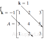
ans=
1
4
3
ans =
2
5
ans =
3
2
Get the elements on the first subdiagonal (k=-1) of A. The result has one fewer element than the main diagonal.
>> x1 = diag(A,-1)
x1 =
10
10
2
9
2
Calling diag twice returns a diagonal matrix composed of the diagonal elements of the original matrix.
>> A1 = diag(diag(A))
A1 =
9 0 0 0 0 0
0 6 0 0 0 0
0 0 9 0 0 0
0 0 0 1 0 0
0 0 0 0 7 0
0 0 0 0 0 9
Magic Matrices
MATLAB includes a matrix function called magic that generates a matrix with unusual properties. In a magic matrix, the sums of the columns are the same, as are the sums of the rows.
>> A = magic(4)
A =
16 2 3 13
5 11 10 8
9 7 6 12
4 14 15 1
>> sum(A)
ans = 34 34 34 34
Not only are the sums of all the columns and rows the same, but the sums of the diagonals are the same.
>> diag(A)
ans =
16
11
6
1
>> sum(diag(A))
ans = 34
Finally, to find the diagonal from lower left to upper right, we first have to “flip” the matrix and then find the sum of the diagonal:
>> fliplr(A)
ans =
13 3 2 16
8 10 11 5
12 6 7 9
1 15 14 4
>> diag(ans)
ans =
13
10
7
4
>> sum(ans)
ans = 34
Practice Exercises 3.2
- Create a 3 × 3 matrix of zeros.
- Create a 3 × 4 matrix of zeros.
- Create a 3 × 3 matrix of ones.
- Create a 5 × 3 matrix of ones.
- Create a 4 × 6 matrix in which all the elements have a value of $\pi $.
- Create a 10 × 10 magic matrix.
- Extract the diagonal from this matrix.
- Extract the diagonal that runs from lower left to upper right from this matrix.
- Confirm that the sums of the rows, columns, and diagonals are all the same.
3.3 Matrix Calculations
Matrix Calculations
Matrix Addition and Subtraction
Matrix Addition and Subtraction
To add, subtract two matrices that are of the same dimensions, it simply adds or subtracts the elements which are in the same position in each matrix.

For example:
>> A = [1 3 1; 1 0 0]; B = [0 0 5; 7 5 1];
>> A + B
ans =
1 3 6
8 5 0
![]()
Scalar Addition/Subtraction
The result of c ± A (or A ± c) is computed by adding/subtracting every entry of A by c:
${\left( {c \pm A} \right)_{i,j}} = c \pm {A_{i,j}}$
>> A + 2
ans =
3 5 3
3 2 2
>> 1 + B
ans =
1 1 6
8 6 2
Difference Dimensions
If two matrices have difference dimensions, make sure they have compatible size. For more information, see Compatible Array Sizes for Basic Operations.
A row vector and a column vector have compatible sizes. If you add a 1×3 vector to a 2×1 vector, then each vector implicitly expands into a 2×3 matrix before MATLAB executes the element-wise addition.
>> x = [1 2 3];
>> y = [10; 15];
>> x + y
ans =
11 12 13
16 17 18
If the sizes of the two operands are incompatible, then you get an error.
>> A = [8 1 6; 3 5 7; 4 9 2];
>> m = [2 4];
>> A - m
Matrix dimensions must agree.
Matrix Multiplication
Matrix Multiplication
The matrix multiplication follows the normal rules of linear algebra. In linear algebra, the product ${A_{[m,n]}} \times {B_{[n,p]}} = {C_{[m,p]}}$ is defined by the equation:
${C_{i,j}} = \sum\limits_{k = 1}^n {{A_{i,k}} \cdot {B_{k,j}}} $
where n is the number of columns on matrix A and the number of rows in matrix B.
Note that for matrix multiplication to work, the number of columns in matrix a must be equal to the number of rows in matrix b.
To multiply an m×n matrix by an n×p matrix, the ns must be the same, and the result is an m×p matrix.
$[m,n] \times [n,p] = [m,p]$
>> A * B
ans =
-5 5
-11 13
Matrix Multiplication is not Commutative
In arithmetic, we are used to: $3 \times 5 = 5 \times 3$ (The commutative low of multiplication).
But this is not generally true for matrices (matrix multiplication is not commutative): $A \times B \ne B \times A$
Matrix Division
Technically, there is no such thing as matrix division. Dividing a matrix by another matrix is an undefined function. The actually divide matrices is:
$A/B = A \times \frac{1}{B} = A \times {B^{ - 1}}$
Where B-1 means the "inverse" of B.
For example:
>> A = [13 26; 39 13]; B = [7 4; 2 3];
>> A / B
ans =
-1.000 10.000
7.000 -5.000
>> A * inv(B)
ans =
-1.000 10.000
7.000 -5.000
Element-by-Element Calculations
Boolean Operations
Boolean Operations
Transposing
Transposing
To "transpose" a matrix, swap the rows and columns.
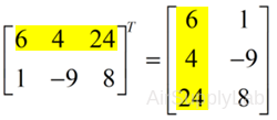
>> X = [6 4 24; 1 -9 8];
>> X'
ans =
6 1
4 -9
24 8
meshgrid Function
[new_x, new_y]=meshgrid(x,y)
The meshgrid command takes the two input vectors and creates two two-dimensional matrices. Each of the resulting matrices has the same number of rows and columns. The number of columns is determined by the number of elements in the x vector, and the number of rows is determined by the number of elements in the y vector. This operation is called mapping the vectors into a two-dimensional array.
Create 2-D grid coordinates with x-coordinates defined by the vector x and y-coordinates defined by the vector y.
>> x = 1:3;
>> y = 1:5;
>> [X,Y] = meshgrid(x,y)
X =
1 2 3
1 2 3
1 2 3
1 2 3
1 2 3
Y =
1 1 1
2 2 2
3 3 3
4 4 4
5 5 5
Evaluate the expression ${x^2} + {y^2}$ over the 2-D grid.
>> X.^2 + Y.^2
ans =
2 5 10
5 8 13
10 13 18
17 20 25
26 29 34
Practice Exercises 3.3
- if $A = \left[ {\begin{array}{ccccccccccccccc} 1&{ - 2}\\ 4&{ - 3} \end{array}} \right]$ and $B = \left[ {\begin{array}{ccccccccccccccc} { - 1}&4\\ 6&{ - 2} \end{array}} \right]$, then what is $3{A^T} - 2{B^T}$ ?
- Using meshgrid to calculate:
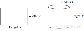
- The area of a rectangle is length times width (area = length × width). Find the areas of rectangles with lengths of 1, 3, and 5 cm and with widths of 2, 4, 6, and 8 cm. (You should have 12 answers.)
- The volume of a circular cylinder is $volume = \pi {r^2}h$.Find the volume of cylindrical containers with radii from 0 to 12 m and heights from 10 to 20 m. Increment the radius dimension by 3 m and the height by 2 m as you span the two ranges.
3.4 Multidimensional Matrices
Two-Dimensional Matrix
Two-Dimensional Matrix
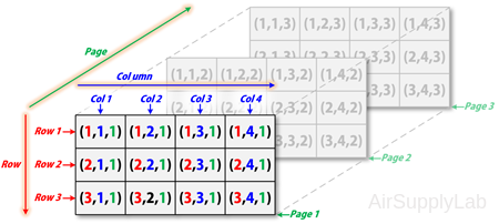
Multidimensional arrays in MATLAB are an extension of the normal two-dimensional matrix. Matrices have two dimensions: the row dimension and the column dimension.
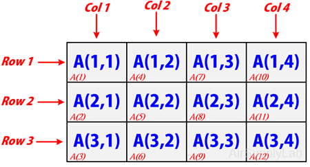
You can access a two-dimensional matrix element with two subscripts: the first representing the row index, and the second representing the column index.
Three-Dimensional Matrix
Three-Dimensional Matrix
Multidimensional arrays use additional subscripts for indexing. A three-dimensional array, for example, uses three subscripts:
- The first references array dimension 1, the row.
- The second references dimension 2, the column.
- The third references dimension 3. This illustration uses the concept of a page to represent dimensions 3 and higher.
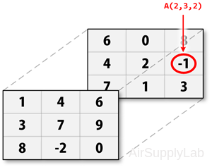
For example, to access the element in the second row, third column of page 2, you can use the subscripts (2,3,2):
Four-Dimensional Matrix
Four-Dimensional Matrix
A four-dimensional matrix has four subscripts:
- The first two reference a row-column pair.
- The second two access the third and fourth dimensions of data.
Creating Multidimensional Matrices
Creating Multidimensional Matrices
You can use the same techniques to create multidimensional arrays that you use for two-dimensional matrices. In addition, MATLAB provides a special concatenation function that is useful for building multidimensional arrays.
There are some methods for creating multidimensional matrices:
- Generating Arrays Using Indexing
- Extending Multidimensional Arrays
- Generating Arrays Using MATLAB Functions
- Building Multidimensional Arrays with the cat Function
Generating Arrays Using Indexing
Generating Arrays Using Indexing
First way to create a multidimensional matrix is to create a two-dimensional matrix and then extend it.
For example, to create an 3×3×2 matrix:
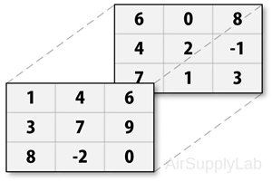
- Create first two-dimensional matrix
>> A = [1 4 6; 3 7 9; 8 -2 0]; - Add a third dimension to matrix A
>> A(:,:,2) = [6 0 8; 4 2 -1; 7 1 3];
>> A
A(:,:,1) =
1 4 6
3 7 9
8 -2 0
A(:,:,2) =
6 0 8
4 2 -1
7 1 3
You can continue to add rows, columns, or pages to the array using similar assignment statements.
Extending Multidimensional Arrays
Extending Multidimensional Arrays
To extend matrix A in any dimension:
- Increment or add the appropriate subscript and assign the desired values.
- Assign the same number of elements to corresponding matrix dimensions. For numeric matrices, all rows must have the same number of elements, all pages must have the same number of rows and columns, and so on.
For example, create an 3×3×3×2 matrix:
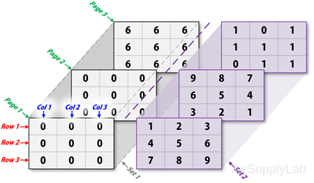
Create an three-dimensional matrix with initial value 0:
>> A = zeros([3 3 3];
A(:,:,1) =
0 0 0
0 0 0
0 0 0
A(:,:,2) =
0 0 0
0 0 0
0 0 0
A(:,:,3) =
0 0 0
0 0 0
0 0 0
Use the MATLAB scalar expression capabilities with the colon operator to fill an entire dimension with a single value:
>> A(:,:,3) = 6
A(:,:,3) =
6 6 6
6 6 6
6 6 6
To turn matrix A from 3×3×3 into a 3×3×3×2 four-dimensional matrix, enter:
>> A(:,:,1,2) = [1 2 3; 4 5 6; 7 8 9];
>> A(:,:,2,2) = [9 8 7; 6 5 4; 3 2 1];
>> A(:,:,3,2) = [1 0 1; 1 1 0; 0 1 1];
Generating Arrays Using MATLAB Functions
Generating Arrays Using MATLAB Functions
You can use MATLAB functions such as randn, ones, and zeros to generate multidimensional matrices in the same way you use them for two-dimensional matrices. Each argument you supply represents the size of the corresponding dimension in the resulting matrices. For example, to create a 4×3×2 matrix of normally distributed random numbers:
>> B = randn(4,3,2)
To generate a matrix filled with a single constant value, use the repmat function. repmat replicates an array (in this case, a 1×1 array) through a vector of array dimensions.
>> B = repmat(5, [3 4 2])
B(:,:,1) =
5 5 5 5
5 5 5 5
5 5 5 5
B(:,:,2) =
5 5 5 5
5 5 5 5
5 5 5 5
Building Multidimensional Arrays with the cat Function
Building Multidimensional Arrays with the cat Function
The cat function is a simple way to build multidimensional arrays; it concatenates a list of arrays along a specified dimension:
>> B = cat(dim, A1, A2...);
where A1, A2, and so on are the arrays to concatenate, and dim is the dimension along which to concatenate the arrays.
For example, to create a new array with cat:
>> B = cat(3, [2 8; 0 5], [1 3; 7 9])
B(:,:,1) =
2 8
0 5
B(:,:,2) =
1 3
7 9
The cat function accepts any combination of existing and new data. In addition, you can nest calls to cat. The lines below, for example, create a four-dimensional array.
>> A = cat(3, [9 2; 6 5], [7 1; 8 4]);
>> B = cat(3, [3 5; 0 1], [5 6; 2 1]);
>> C = cat(4, A, B, cat(3, [1 2; 3 4], [4 3;2 1]));
cat automatically adds subscripts of 1 between dimensions, if necessary. For example, to create a 2×2×1×2 array, enter
>> D = cat(4, [1 2; 4 5], [7 8; 3 2])
D(:,:,1,1) =
1 2
4 5
D(:,:,1,2) =
7 8
3 2
In the previous case, cat inserts as many singleton dimensions as needed to create a four-dimensional array whose last dimension is not a singleton dimension. If the dim argument had been 5, the previous statement would have produced a 2×2×1×1×2 array. This adds additional 1s to indexing expressions for the array. To access the value 8 in the four-dimensional case, use
>> D(1,2,1,2) # The third subscript '1' means single dimension index
D = 8
Any dimension of a matrix can have size zero, making it a form of empty array. For example, 10×0×20 is a valid size for a multidimensional matrix.
>> A = ones([10 0 20]);
A = 10×0×20 empty double array
Questions
- Create the following matrices, and use them in the exercises that follow:
$A = \left[ {\begin{array}{ccccccccccccccc} {15}&3&{22}\\ 3&8&5\\ {14}&3&{82} \end{array}} \right]$$B = \left[ {\begin{array}{ccccccccccccccc} 1\\ 5\\ 6 \end{array}} \right]$$C = \left[ {\begin{array}{ccccccccccccccc} {12}&{18}&5&2 \end{array}} \right]$- Create a matrix called D from the third column of matrix A.
- Combine matrix B and matrix D to create matrix E, a two-dimensional matrix with three rows and two columns.
- Combine matrix B and matrix D to create matrix F, a one-dimensional matrix with six rows and one column.
- Create a matrix G from matrix A and the first three elements of matrix C, with four rows and three columns.
- Create a matrix H with the first element equal to A1,3, the second element equal to C1,2, and the third element equal to B2,1.
- Create a 6×6 magic matrix.
- What is the sum of each of the rows?
- What is the sum of each of the columns?
- What is the sum of each of the diagonals?
- The ideal gas law, $Pv = RT$, describes the behavior of many gases. When solved for v (the specific volume, m3 /kg), the equation can be written
$v = \frac{{RT}}{P}$
Find the specifi c volume for air, for temperatures from 100 to 1000 K and for pressures from 100 kPa to 1000 kPa. The value of R for air is 0.2870 kJ/(kg K).
In this formulation of the ideal gas law, R is different for every gas. There are other formulations in which R is a constant, and the molecular weight of the gas must be included in the calculation. You’ll learn more about this equation in chemistry classes and thermodynamics classes. Your answer should be a two-dimensional matrix.
